Given the current SARS-CoV2 pandemic, expressions and models from the field of epidemiology are frequently discussed in the media. To get a better understanding of the terms, it is quite helpful to have a look at one of the models, which is called the Reed-Frost Model after its inventors or Chain Binomial Model after the mathematical structure it follows. It is a rather simple model in discrete time which makes strong assumptions and is hence limited in its significance. Nevertheless it is very helpful to get a basic understanding of some of the underlying concepts for other models as well. The following is losely based on "Mathematical Modeling in Epidemiology" by J.C. Frauenthal, which can be bought used and is a reading recommendation. We make the following assumptions:
Time is discrete. The incubation time (also called latency) is exactly one time step in duration. This means, that all infections are passed in every time step. Also, the infection only lasts one time step.
Population Size is constant \(N\). The population consists of three types:
Susceptible \(S_n\), the individuals which are suceptible for the disease at time \(n\),
Infected \(I_n\), the infected individuals at tme \(n\), which can spread the disease,
Removed \(R_n\), the individuals which cannot be infected at time \(n\), because they developed immunity.
These groups, from which the population is constructed, give this type of models the name "SIR-model". It follows, that the transition will only be in the direction \(S_n \to I_n \to R_n\), which means, that all infected will be rendered immune. It follows, that \(S_n + I_n + R_n = N\) will always be fulfilled.
The probability, that a susceptible individual catches the disease from a particular infected in one time step is given by \(p\). The probability that this susceptible does not get infected from any of the \(I_n\) infected in time step \(n\) is hence given by \[\begin{aligned} Q_n = (1-p)^{I_n} =: q^{I_n}.\end{aligned}\] If we want to have a look at the probability, that there are exactly \(I\) infected at time \(n+1\), we need to take a look at the conditional probability \(\mathbb{P}\left(S_{n+1} = S_n-I, I_{n+1} = I \vert S_n, I_n \right)\) which is the probability, that from the \(S_n\) susceptibel individuals exactly \(I\) will be infected in the next time step, given, that we had \(I_n\) infected in this time step: \[\begin{aligned} \mathbb{P}\left(S_{n+1} = S_n-I, I_{n+1} = I \vert S_n, I_n \right) &=\#_{\text{pick $I$ from $S_n$}} \cdot \mathbb{P}(S_n-I \text{ not infected}) \cdot \mathbb{P}(I \text{ infected})\\ &= \binom{S_n}{I} Q_n ^{S_n -I} (1-Q_n)^I =: \mathbb{P}(I), \end{aligned}\] which is a binomial distribution. To calculate the average number of infected we need some identities concerning the binomial coefficient. The binomial identity is given by \[\begin{aligned} \sum_{n=0}^N \binom N n x^n y^{N-n} = (x+y)^N. \end{aligned}\]
We will also need, that \[\begin{aligned} \binom N n &= \frac{N!}{n! (N-n)!}\\ &=\frac{N}{n} \frac{(N-1)!}{(n-1)!\left( (N-1) - (n-1)\right)!}\\ &=\frac{N}{n} \binom{N-1}{n-1}. \end{aligned}\] To calculate the expected value for given \(S_n\) and \(Q_n\) we need to calculate \[\begin{aligned} \langle I_{n+1} \rangle_{S_n, Q_n} &= \sum_{I = 0}^{S_n} I \mathbb{P}\\ &= \sum_{I = 0}^{S_n} I \binom{S_n}{I} Q_n ^{S_n -I} (1-Q_n)^I\\ &= \sum_{I = 0}^{S_n} I \frac{S_n}{I}\binom{S_n-1}{I-1} Q_n ^{S_n -I} (1-Q_n)(1-Q_n)^{I-1}\\ &\stackrel{I\to I+1}{=} S_n(1-Q_n) \sum_{I = 0}^{S_n-1} \binom{S_n-1}{I} Q_n ^{S_n -1 -I} (1-Q_n)^{I}\\ &= S_n(1-Q_n) \cdot (Q_n + 1 - Q_n)^{S_n-1}\\ &= S_n(1-Q_n).\end{aligned}\]
Knowing, that \(S_{n+1} = S_n - I_{n+1}\) it follows directly, that \[\begin{aligned} \langle S_{n+1} \rangle_{S_n, Q_n} &= \langle S_n - I_{n+1}\rangle_{S_n, Q_n}\\ &=\langle S_n\rangle_{S_n, Q_n} - \langle I_{n+1}\rangle_{S_n, Q_n} = S_n - S_n(1-Q_n)\\ &= S_n Q_n.\end{aligned}\]
Although this seems to be a nice expression, keep in mind, that it is still the conditional expected value for one time step only. What is really of interest is the unconditioned value: independent of the previous time step, so that we can make some statements about the general behaviour of the epidemic. Sadly, this is not nice to calculate. Of course, we can set the starting conditions \(S_0\) and \(I_0\). It then follows, that \[\begin{aligned} \mathbb{P}(S_1) &= \mathbb{P}\left(S_{1} = S_0-I, I_{1} = I \vert S_0, I_0 \right)\\ \mathbb{P}(S_2) &= \sum_{S_1, I_1} \sum_{I = 0}^{S_1} \mathbb{P}(S_1, I_1\vert S_0, I_0)\mathbb{P}\left(S_{2} = S_1-I, I_{2} = I \vert S_1, I_1 \right)\\ \dots&\\ \mathbb{P}(S_n) &= \sum_{S_1, I_1}\dots \sum_{S_n, I_n} \sum_{I = 0}^{S_n} \prod_{i=1}^{n-1}\mathbb{P}(S_i, I_i\vert S_{i-1}, I_{i-1})\mathbb{P}\left(S_{n} = S_{n-1}-I, I_{n} = I \vert S_{n-1}, I_{n-1} \right)\end{aligned}\] which looks pretty messy already in the second time step and no doubt does not look like fun in he general expression. Also keep in mind, that this needs to be calculated for every set of starting conditions you are interested in.
It is much more fun to simulate the infection dynamics. We will be doing it as follows, starting with fixing the starting condiitons \(N\), \(I_0\) and \(S_0\):
Calculate all \(\mathbb{P}(S_1 = S_0-I, I)\) for \(I \in \{0, \dots, S_0\}\) and remember, that \(\sum_{I}\mathbb{P}(S_1 = S_0-I, I) = 1\).
Partition a unit interval according to \(\{\mathbb{P}(S_1 = S_0-I, I)\}\)
Draw a random number \(X \in (0, 1)\) and see to which Probability \(\mathbb{P}(S_1 = S_0-I, I)\) it corresponds
Use this to choose new \(S\) and \(I\) values
Update the time and start over until \(S_n = 0\) (population completely immune) or \(I=0\) (disease died out).
My implementation was done in C++ and for the random numbers GSL was used. The code can be found at my gitlab. The plotting was done with gnuplot.
This simple model can already give some insight into the dynamics of an epidemic. To show two very important effencts the following Plots show four situations: Two different group sizes (called population size) of 50 and 150 individuals and two different values for \(p\) of 0.05 and 0.01.
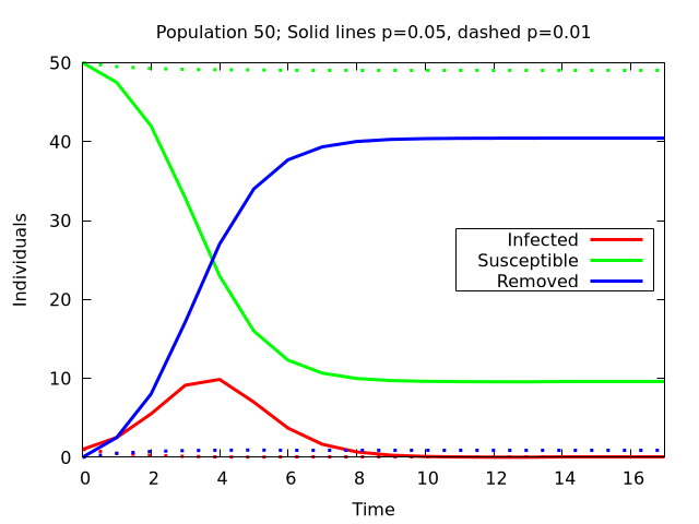
With 50 Susceptible individuals and one infected at starting time the solid lines are results for \(p = 0.05\) and the dashed ones are for \(p = 0.01\). It is very obvious, that the infections are drastically reduced for the lower value. Much more than the factor 5 by which \(p\) is reduced.
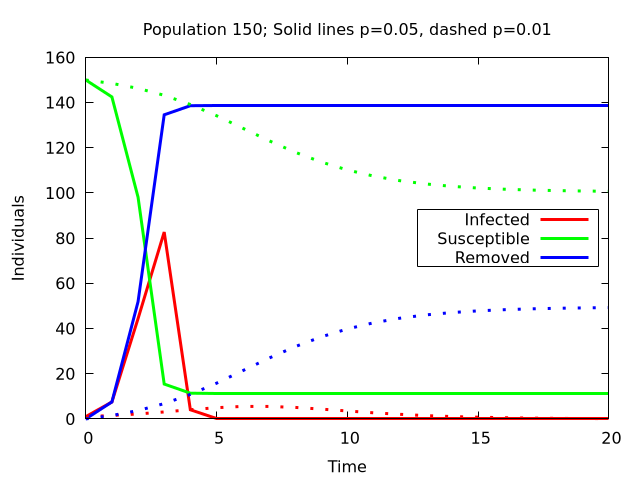
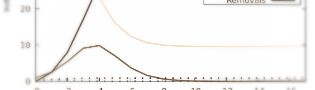
In the larger population the infection spreads much faster. The number of infections peaks already at \(t=3\) in the case of \(p=0.05\). Again, reducing \(p\) has a huge impact on the dynamics. Although the infection is not reduced as heavily as in the smaller population, it is slowed down by a lot and the number of removed stagnate at around 50 in contrast to 150 in the larger group.
Lessons learned
What is to be learned from such an immensely simplified model as the presented realization of a Reed-Frost-Model? Well for one it can be learned, that the modeling of epidemics is very difficult. Even for the simple, deterministic model as presented here, a simulation is preferred to the evaluation of the exact term. On the other hand two of the main messages of the science community on the topic are very obvious in the results of my simulations:
Reduce the amount of contacts to other people to a minimum. This is what the different group sizes tell us. As we go from 50 to 150 individuals in the simulation the disease gains momentum. There are much more infections in much shorter times. This would result in a much higher stress on the health system and should be avoided under all circumstances.
Reduce \(p\). Well this one is not as clear as the last statement because \(p\) is not defined properly. It is more of a combined value of contact probability, attack rate, etc. But the obvious interpretation would be: Do everything to make an infection less likely. Wear a mask, open the windows, keep your distance, wash your hands.